13. Stochastic Short Rates
This brief section illustrates the use of stochastic short rate models for simulation and (risk-neutral) discounting. The class used is called stochastic_short_rate.
13.1. The Modelling
First, the market environment. As a stochastic short rate model the square_root_diffusion class is (currently) available. We therefore need to define the respective parameters for this class in the market environment.
[1]:
from dx import *
[2]:
me = market_environment(name='me', pricing_date=dt.datetime(2015, 1, 1))
me.add_constant('initial_value', 0.01)
me.add_constant('volatility', 0.1)
me.add_constant('kappa', 2.0)
me.add_constant('theta', 0.05)
me.add_constant('paths', 1000)
me.add_constant('frequency', 'M')
me.add_constant('starting_date', me.pricing_date)
me.add_constant('final_date', dt.datetime(2015, 12, 31))
me.add_curve('discount_curve', 0.0)  # dummy
me.add_constant('currency', 0.0)  # dummy
Second, the instantiation of the class.
[3]:
ssr = stochastic_short_rate('sr', me)
The following is an example list object containing datetime objects.
[4]:
time_list = [dt.datetime(2015, 1, 1),
             dt.datetime(2015, 4, 1),
             dt.datetime(2015, 6, 15),
             dt.datetime(2015, 10, 21)]
The call of the method get_forward_reates() yields the above time_list object and the simulated forward rates. In this case, 10 simulations.
[5]:
ssr.get_forward_rates(time_list, 10)
[5]:
([datetime.datetime(2015, 1, 1, 0, 0),
  datetime.datetime(2015, 4, 1, 0, 0),
  datetime.datetime(2015, 6, 15, 0, 0),
  datetime.datetime(2015, 10, 21, 0, 0)],
 array([[0.01      , 0.01      , 0.01      , 0.01      , 0.01      ,
         0.01      , 0.01      , 0.01      , 0.01      , 0.01      ],
        [0.03277202, 0.02888579, 0.02597219, 0.03437966, 0.02609197,
         0.02668004, 0.03056627, 0.03347986, 0.02507239, 0.03336008],
        [0.04847622, 0.02778153, 0.02208502, 0.03542504, 0.03381398,
         0.02848213, 0.04861457, 0.05589349, 0.03990585, 0.04257658],
        [0.05166403, 0.04121302, 0.05144506, 0.06797319, 0.02824299,
         0.0419498 , 0.05243283, 0.03619928, 0.02328994, 0.06677311]]))
Accordingly, the call of the get_discount_factors() method yields simulated zero-coupon bond prices for the time grid.
[6]:
ssr.get_discount_factors(time_list, 10)
[6]:
([datetime.datetime(2015, 1, 1, 0, 0),
  datetime.datetime(2015, 4, 1, 0, 0),
  datetime.datetime(2015, 6, 15, 0, 0),
  datetime.datetime(2015, 10, 21, 0, 0)],
 array([[0.96930155, 0.97754222, 0.97798078, 0.9696954 , 0.97874354,
         0.97771286, 0.96961689, 0.96977567, 0.97816125, 0.96819563],
        [0.97442643, 0.98223994, 0.98232769, 0.97501559, 0.98310835,
         0.98214428, 0.97447841, 0.97498814, 0.98239997, 0.97338523],
        [0.98259442, 0.98797521, 0.98718981, 0.98203326, 0.98917777,
         0.98772624, 0.98243814, 0.9839819 , 0.98898026, 0.981009  ],
        [1.        , 1.        , 1.        , 1.        , 1.        ,
         1.        , 1.        , 1.        , 1.        , 1.        ]]))
13.2. Stochstic Drifts
Let us value use the stochastic short rate model to simulate a geometric Brownian motion with stochastic short rate. Define the market environment as follows:
[7]:
me.add_constant('initial_value', 36.)
me.add_constant('volatility', 0.2)
  # time horizon for the simulation
me.add_constant('currency', 'EUR')
me.add_constant('frequency', 'M')
  # monthly frequency; paramter accorind to pandas convention
me.add_constant('paths', 10)
  # number of paths for simulation
Then add the stochastic_short_rate object as discount curve.
[8]:
me.add_curve('discount_curve', ssr)
Finally, instantiate the geometric_brownian_motion object.
[9]:
gbm = geometric_brownian_motion('gbm', me)
We get simulated instrument values as usual via the get_instrument_values() method.
[10]:
gbm.get_instrument_values()
[10]:
array([[36.        , 36.        , 36.        , 36.        , 36.        ,
        36.        , 36.        , 36.        , 36.        , 36.        ],
       [36.8060297 , 35.75560124, 34.98778226, 37.24953986, 35.01902026,
        35.17279091, 36.20609756, 37.00065288, 34.75400748, 36.96764721],
       [38.21614839, 34.16569133, 32.70350696, 36.40954077, 34.65561565,
        33.87070953, 37.88603564, 39.58040249, 35.55090852, 37.35044144],
       [38.47450027, 33.88999526, 34.0982215 , 39.27489627, 32.69322908,
        33.66728041, 38.22119959, 37.9877562 , 32.97984662, 39.62076877],
       [37.76574157, 33.70921262, 34.93754066, 41.4857547 , 33.30286899,
        34.3470077 , 38.48001428, 37.12512733, 31.26650887, 38.95014155],
       [41.40824335, 32.65237919, 34.18828508, 39.57699414, 36.64649108,
        31.39011407, 39.80780981, 38.01482674, 32.84186281, 35.46744615],
       [41.32002568, 32.83888512, 33.57945454, 39.52883894, 36.05892171,
        31.53555452, 39.68092784, 38.79866413, 32.96181069, 36.13177382],
       [46.41216195, 32.72457065, 32.48000699, 35.96872893, 38.02757568,
        28.16218767, 39.93935721, 40.23115152, 36.33000552, 34.36135112],
       [43.76336092, 34.05939936, 38.16985125, 37.76248586, 35.7087264 ,
        29.96841401, 38.50269177, 34.34515834, 34.71596345, 36.71192144],
       [43.41102129, 33.28842046, 37.53369604, 35.44705255, 34.25211077,
        30.3159961 , 39.53272861, 35.04339421, 37.10939043, 38.4034044 ],
       [50.70091956, 35.54130837, 33.67719457, 34.15617789, 36.58057258,
        26.05844606, 37.16975856, 39.1972456 , 38.65893079, 36.09388287],
       [51.40881852, 33.92751964, 30.54827552, 36.53604564, 38.97303122,
        25.80445233, 39.08967422, 43.37205968, 36.28052847, 34.0082156 ],
       [45.46321155, 31.21544356, 30.90125559, 39.76590057, 39.76247076,
        29.30040939, 42.66414473, 43.05146618, 33.47040857, 33.47267446]])
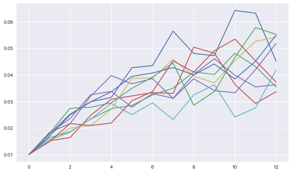
13.3. Visualization of Simulated Stochastic Short Rate
[11]:
from pylab import plt
plt.style.use('seaborn')
%matplotlib inline
[12]:
# short rate paths
plt.figure(figsize=(10, 6))
plt.plot(ssr.process.instrument_values[:, :10]);
Copyright, License & Disclaimer
© Dr. Yves J. Hilpisch | The Python Quants GmbH
DX Analytics (the “dx library” or “dx package”) is licensed under the GNU Affero General Public License version 3 or later (see http://www.gnu.org/licenses/).
DX Analytics comes with no representations or warranties, to the extent permitted by applicable law.
http://tpq.io | dx@tpq.io | http://twitter.com/dyjh
Quant Platform | http://pqp.io
Python for Finance Training | http://training.tpq.io
Certificate in Computational Finance | http://compfinance.tpq.io
Derivatives Analytics with Python (Wiley Finance) | http://dawp.tpq.io
Python for Finance (2nd ed., O’Reilly) | http://py4fi.tpq.io